Author: Vikranth Srivatsa, Zijian He, Pu Guo, Dongming Li, and Yiying Zhang
TLDR: A single LLM deployment now serves everything from latency-critical chat to relaxed background jobs under a fixed GPU budget, creating a tiered-SLO serving problem. We designed Nitsum [arXiv ‘26], the first serving system that treats tensor parallelism (TP) as a runtime control surface instead of a fixed deployment choice. By making TP switching nearly free and continuously reconfiguring the cluster to track shifting workloads, Nitsum improves SLO-compliant goodput by up to 5.3x over state-of-the-art serving systems.
LLM Serving Is Increasingly Tiered
A single model deployment today serves a mix of very different workloads on the same infrastructure: interactive chat, coding agents, computer-use agents, API calls embedded in products, and long-running background or scheduled jobs. Their latency expectations differ widely. Some need a fast first token and a steady token rate for a human in the loop; others tolerate much slower responses in exchange for lower cost. In practice, this creates tiers of service objectives.
Serving one request happens in two phases. First comes prefill: the model reads the entire prompt and produces the first token. Then comes decode: it generates the rest of the answer one token at a time. These two phases map directly to the two latency targets, called service-level objectives (SLOs), that users care about: Time To First Token (TTFT), set by prefill, and Time Per Output Token (TPOT), set by decode. A request only “counts” toward goodput if it meets both its TTFT and TPOT targets. With unlimited GPUs, tiered serving would be easy: give each tier its own cluster. But providers run under fixed GPU budgets, and the workload mix, request lengths, and load intensity all vary substantially over time. Strictly separating clusters wastes capacity; pooling all requests together makes the heterogeneous TTFT and TPOT objectives interfere.
This leads to the central question of our work:
How should an LLM serving system operate under a fixed GPU budget and maximize the number of requests per second that meet both their TTFT and TPOT SLOs (i.e., goodput) for multiple SLO tiers?
Tensor Parallelism Is a Hidden SLO Knob
First, what is tensor parallelism? A large model is too big for one GPU, so tensor parallelism (TP) splits each layer’s weight matrices across N GPUs. The GPUs work on every token together, exchanging partial results over a fast interconnect at each step. TP is normally set once, just high enough to make the model fit, and then never touched.
Existing SLO-aware systems mostly control when requests run: queuing, batching, migration, autoscaling. They leave how each request executes largely fixed. Our key observation is that the execution configuration itself can be used to improve SLO attainment, and the TP level, usually treated as a fixed deployment setting, is one of the most powerful knobs available.
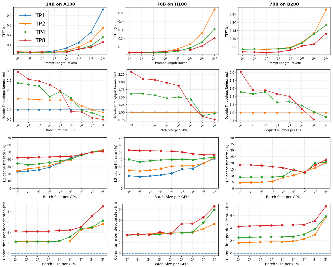
Figure 2: Effect of tensor parallelism on TTFT, decode throughput, L2 cache hit rate, and communication cost across 14B and 70B models on A100, H100, and B200.
Higher TP splits the prefill work across more GPUs, so it reduces prefill latency and improves TTFT, which helps for long prompts or tight first-token targets. Decode is less obvious. When only a few requests are being processed at once, higher TP can also raise decode throughput, and therefore improve TPOT, by up to 3x. That looks backwards, since adding GPUs adds cross-GPU communication. The cause turns out to be memory rather than communication. At low TP, each GPU has to stream a huge weight matrix out of slow GPU memory on every decode step. At higher TP, each GPU holds a smaller slice that fits in its fast on-chip cache, so it spends much less time waiting on memory. Below a certain batch size that memory saving outweighs the extra communication; above it, communication dominates and lower TP is better. So TP affects both TTFT and TPOT, which makes it a usable runtime knob and not only a deployment choice.
No Single Static TP Wins
Because TP affects prefill and decode differently, and because each SLO tier imposes its own latency pressure, the goodput-optimal configuration is not fixed; it shifts as the workload mix and load change over time.
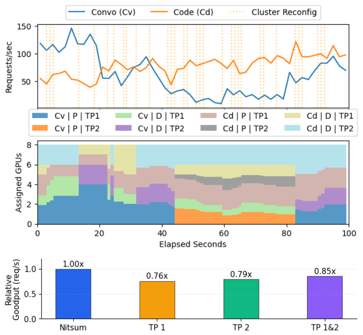
Figure 1: ServeGen conversation and coding workloads on 8 H100 GPUs. Request demand and the optimal cluster configuration vary continuously; no single static TP setting achieves the best goodput.
Figure 1 shows this on a real production trace (ServeGen, calibrated to Alibaba Cloud Model Studio): demand swings continuously and the GPU allocation has to chase it. Figure 3 puts a number on the cost of not chasing it. An oracle that re-picks the best configuration at each step beats every static TP choice by 23–29%.
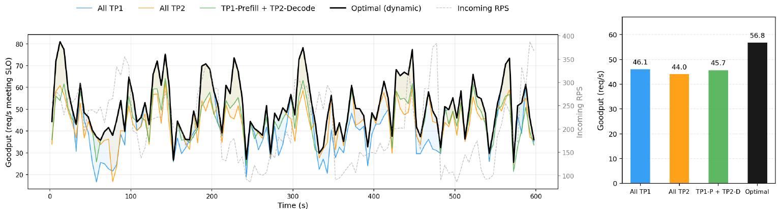
Figure 3: Per-second goodput for three static TP baselines vs. an oracle that selects the best configuration at each step. No static configuration dominates across time; dynamic adaptation yields 23–29% higher aggregate goodput.
The problem is that naively changing TP at runtime means reloading the weights, rebuilding the GPU code, and shuffling each request’s saved state across GPUs. That can take seconds to tens of seconds, comparable to or longer than the workload bursts themselves. Today’s systems end up spending most of their time reconfiguring instead of serving. The central challenge is to make execution-level TP adaptation fast enough to track workload dynamics.
Introducing Nitsum
Nitsum is a distributed LLM serving system that treats TP as an almost-free runtime control surface. It combines three pieces: (1) low-overhead TP-switching mechanisms, (2) a goodput-aware cluster reconfiguration policy, and (3) SLO-aware request scheduling, all coordinated by global and local schedulers. We cover the switching mechanisms next, then the reconfiguration and scheduling policy.
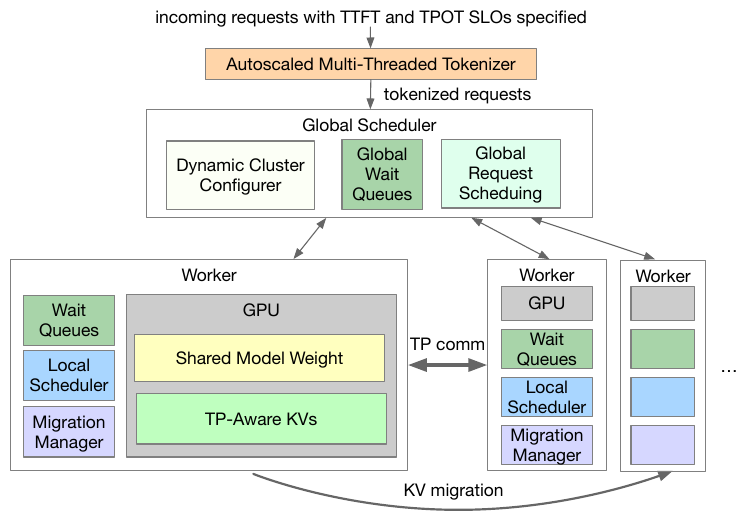
Figure 4: Nitsum architecture. A global scheduler handles cluster configuration, global wait queues, and request scheduling; workers hold a shared model weight and TP-aware KVs, with KV migration between them.
Zero-Overhead TP Weight Switching
With traditional TP, a model’s weights are sharded across GPUs, so changing the TP level means rebuilding the weight matrix. For a 14B model that takes about 30 seconds, plus extra time to rebuild and warm up the GPU code. Keeping a pre-split copy for every TP level avoids the reload but burns memory (45.5 GB for a 13B Llama, about 56% of an A100/H100).
Nitsum instead keeps one full copy of the model weights on each GPU and, at run time, picks out just the slice a given TP level needs using customized GPU kernels (the low-level functions that run on the GPU). Building and warming up these kernels is itself slow, so Nitsum pre-launches a warm process for every candidate TP level ahead of time, each already specialized to its layout, and keeps the inactive ones hibernated with lightweight keep-alive signals. A TP switch then just wakes up an already-warm process, with no on-the-fly profiling or compilation.
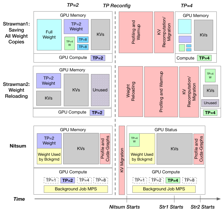
Figure 5: Comparison of Nitsum and straw-man TP weight loading. Straw-man 1 (all weight copies) and 2 (weight reloading) incur profiling/warmup/migration stalls; Nitsum keeps processes pre-allocated and warm.
Aggregated and Pipelined KV Migration
As the model generates, it saves the attention state for every token it has already seen. This saved state is the KV cache, and it means the model never has to re-read the prompt from scratch. The cache is large, lives on the GPU, and is split across the TP GPUs. So when the TP level changes, the KV cache of every request still being processed has to be re-split and shuffled onto the new set of GPUs.
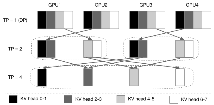
Figure 6: KV conversion in Nitsum when changing from TP 1 to TP 2 to TP 4 on a cluster of four GPUs and 8 KV heads.
Modern systems store this cache in many small fixed-size blocks scattered across GPU memory (a scheme called PagedAttention), so one request’s cache is spread over lots of non-contiguous chunks. The standard GPU copy call (cudaMemcpyAsync) then fires off a separate transfer per chunk, which means thousands of tiny transfers and high latency. Nitsum’s custom migration kernel instead first gathers the scattered chunks into one contiguous buffer, then overlaps that gathering with the network transfer (a technique called pipelining) using a pair of small buffers, so copying and sending happen at the same time.
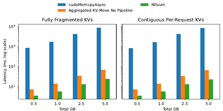
Figure 7: KV-migration latency (log scale) across payload sizes. Nitsum reduces migration latency by 245x–376x vs. cudaMemcpyAsync — 3.6 to 24.8 ms total.
With migration overhead this low, Nitsum can afford a simple stop-and-migrate approach: pause forwarding, migrate KVs, and resume in the new TP level. The whole reconfiguration finishes in under a second.
The Scheduling Policy
Cheap TP switching only helps if the system knows what to switch to. Nitsum’s second core contribution is a full policy for dynamic cluster reconfiguration and SLO-aware request scheduling, run by a lightweight Rust-based global scheduler plus per-GPU local schedulers. It has two halves: deciding the cluster configuration each control window, and routing individual requests to GPUs.
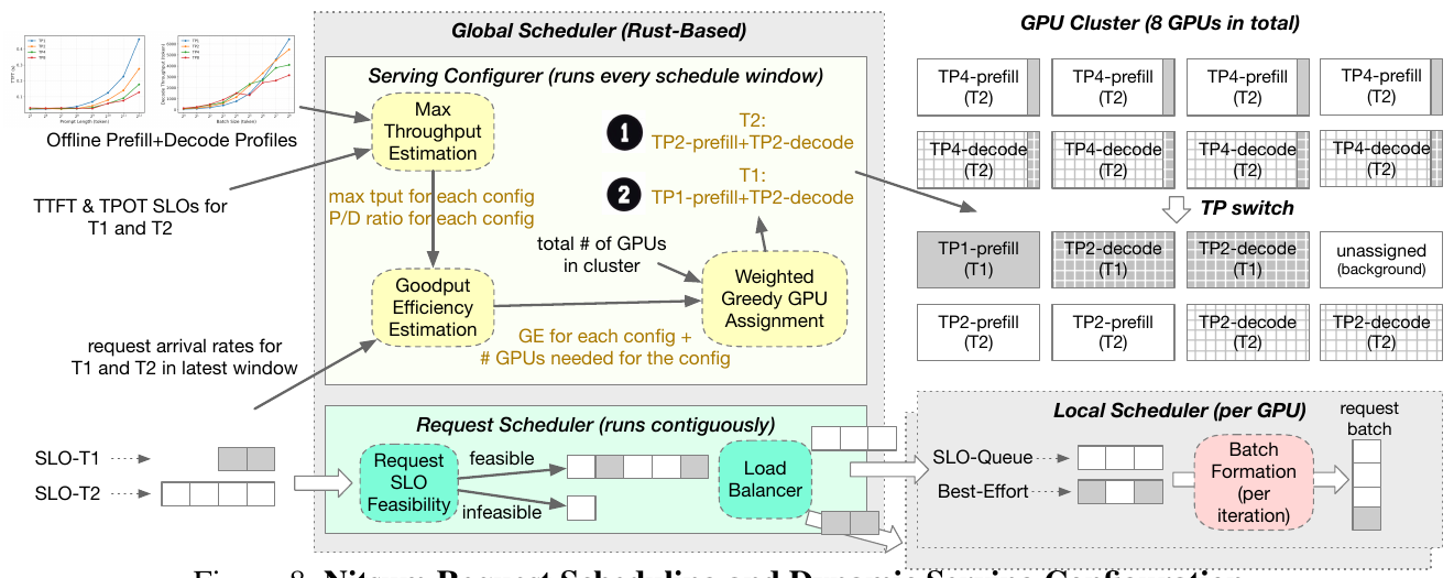
Figure 8: Nitsum's request scheduling and dynamic serving configuration. A serving configurator runs every window to pick TP levels and prefill/decode GPU allocation; a request scheduler runs continuously to place feasible and best-effort requests.
Goodput-Aware Cluster Reconfiguration
Every control window (default one second), Nitsum’s global scheduler picks a new cluster configuration: how many GPUs each SLO tier gets, the TP level for each, and the prefill/decode split. The goal is to maximize goodput efficiency, meaning SLO-compliant throughput per GPU, subject to fairness across tiers.
It does this in two stages. First, estimate how good each configuration is. Using the offline profiles from Figure 2, the scheduler knows the highest request rate a given TP level can serve without breaking that tier’s TTFT/TPOT SLOs. It scores each configuration by a simple ratio:
goodput efficiency = (SLO-compliant requests/sec it can actually serve) ÷ (GPUs it uses)
The throughput is capped by how many requests are actually arriving, since a configuration can’t earn credit for load it never receives.
Second, assign GPUs greedily but fairly. The number of possible configurations (tier × TP level × prefill/decode split) explodes combinatorially, so Nitsum hands GPUs out one group at a time to whichever configuration gives the biggest improvement. A pure greedy step would starve a tier that happens to be less efficient, so Nitsum first multiplies each tier’s score by how starved it currently is (arriving requests ÷ served requests), which keeps the allocation efficient while staying fair. Searching every configuration stays affordable for two reasons: the multi-threaded Rust scheduler does it in about 2.5 ms even at 128 GPUs, and millisecond TP switching means whatever it picks can actually be applied.
SLO-Aware Request Scheduling
Between reconfigurations, the global scheduler routes incoming requests first-come-first-served. For each GPU it tracks how much SLO-safe capacity is left, defined as the most that GPU’s tier can handle minus what is already promised to requests in progress. If a new request fits, it is feasible and sent to the least-loaded GPU of its tier. If it would blow the budget, or if it is an explicit background job, it becomes best-effort work and is spread round-robin across GPUs so no spare capacity is wasted.
Each GPU then runs its own local scheduler with separate queues for feasible, best-effort, and background requests. On every model step it builds a batch sized to stay within its tier’s SLO-safe throughput, fills it with feasible requests first, and only then tops it up with best-effort work. When a request finishes, the GPU reports back so the capacity bookkeeping stays accurate. Together, the reconfiguration policy and this scheduler let Nitsum convert cheap TP switching into real tracking of shifting, multi-tier workloads.
Results
Nitsum is implemented on top of SGLang, rewriting its global scheduler, local scheduler, GPU kernels, and KV-migration mechanism, about 12K source lines in total. We evaluate it against five baselines (Llumnix, Chiron, a separated per-SLO-tier cluster called Split, SGLang with prefill and decode run on separate GPUs, and vanilla SGLang) on two GPU types (A100, H100), two models (Llama 8B, 14B), two cluster sizes, and two production traces (Azure and ServeGen). Load is measured in requests per second (RPS).
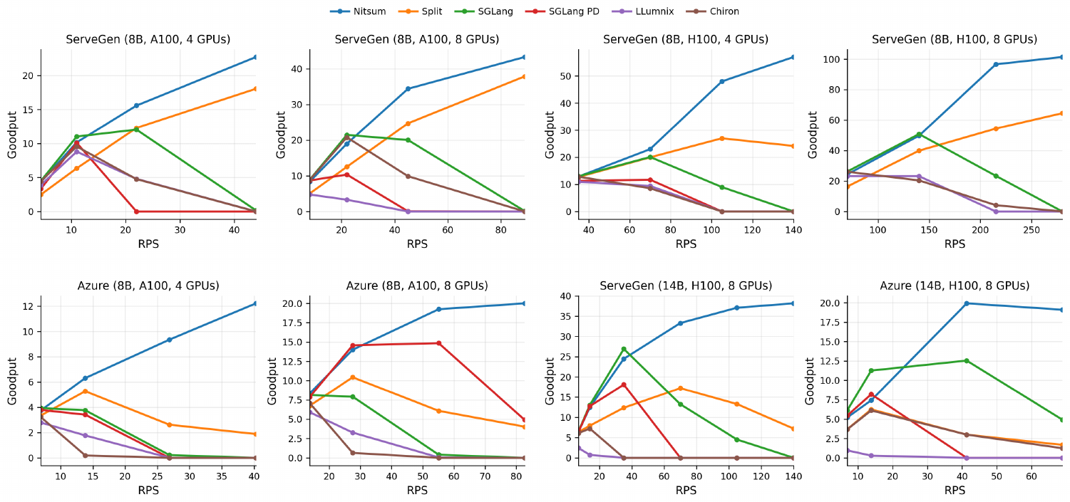
Figure 9: Goodput across two production traces, two GPU types, two cluster sizes, and two model sizes. Nitsum achieves the highest goodput, and is the only system whose goodput consistently increases with load.
Nitsum reaches the highest goodput of all the systems, especially at high load, and it is the only one whose goodput keeps rising as load grows. Against the strongest baseline in each setting it delivers up to 5.3x higher goodput, and the gap widens as load rises. Most baselines collapse at some point. For the 8B model on 4 A100 GPUs, every baseline except Split drops to zero goodput beyond 40 RPS, while Nitsum keeps serving. Across all settings Nitsum holds both TTFT and TPOT below their SLOs while most baselines violate one or both, and its average latency stays comparable to or better than the baselines.
An ablation isolates where the gains come from:
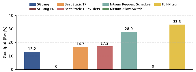
Figure 12: Progressively adding Nitsum's mechanisms (14B on 8 H100, 70 RPS). Dynamic TP only helps when paired with low-overhead switching — slow switching brings goodput to zero.
Vanilla SGLang reaches 13.2 req/s. Adding SLO-aware scheduling with the best static TP gets to 16.7, and separating tiers barely helps (17.2). Nitsum’s SLO-aware scheduler raises this to 28.0. Adding dynamic TP with naive (slow) switching collapses goodput back to zero, which confirms that low-latency switching is essential. The full Nitsum system reaches 33.3 req/s, so dynamic parallelism adaptation delivers its largest gains only when paired with efficient switching.
Our Vision
LLM deployments increasingly have to serve many service tiers from one fixed GPU budget. Most serving systems treat the model’s execution configuration as fixed and only schedule requests around it. Nitsum shows that the execution configuration can be a runtime resource too. Tensor parallelism is the first knob we make cheap enough to change on the fly, and we expect the same approach to apply to other execution choices, such as the prefill/decode split or the quantization level. As real workloads get more heterogeneous and bursty, cheaply reconfiguring how the model runs will matter as much as scheduling when requests run, and we think it is a promising direction for the next generation of serving systems.
If you use Nitsum for your research, please cite our paper:
@misc{srivatsa2026nitsum,
  title="{Nitsum: Serving Tiered LLM Requests with Adaptive Tensor Parallelism}",
  author={Vikranth Srivatsa and Zijian He and Pu Guo and Dongming Li and Yiying Zhang},
  year={2026},
  eprint={2605.05467},
  archivePrefix={arXiv},
  primaryClass={cs.DC},
  url={https://arxiv.org/abs/2605.05467},
}